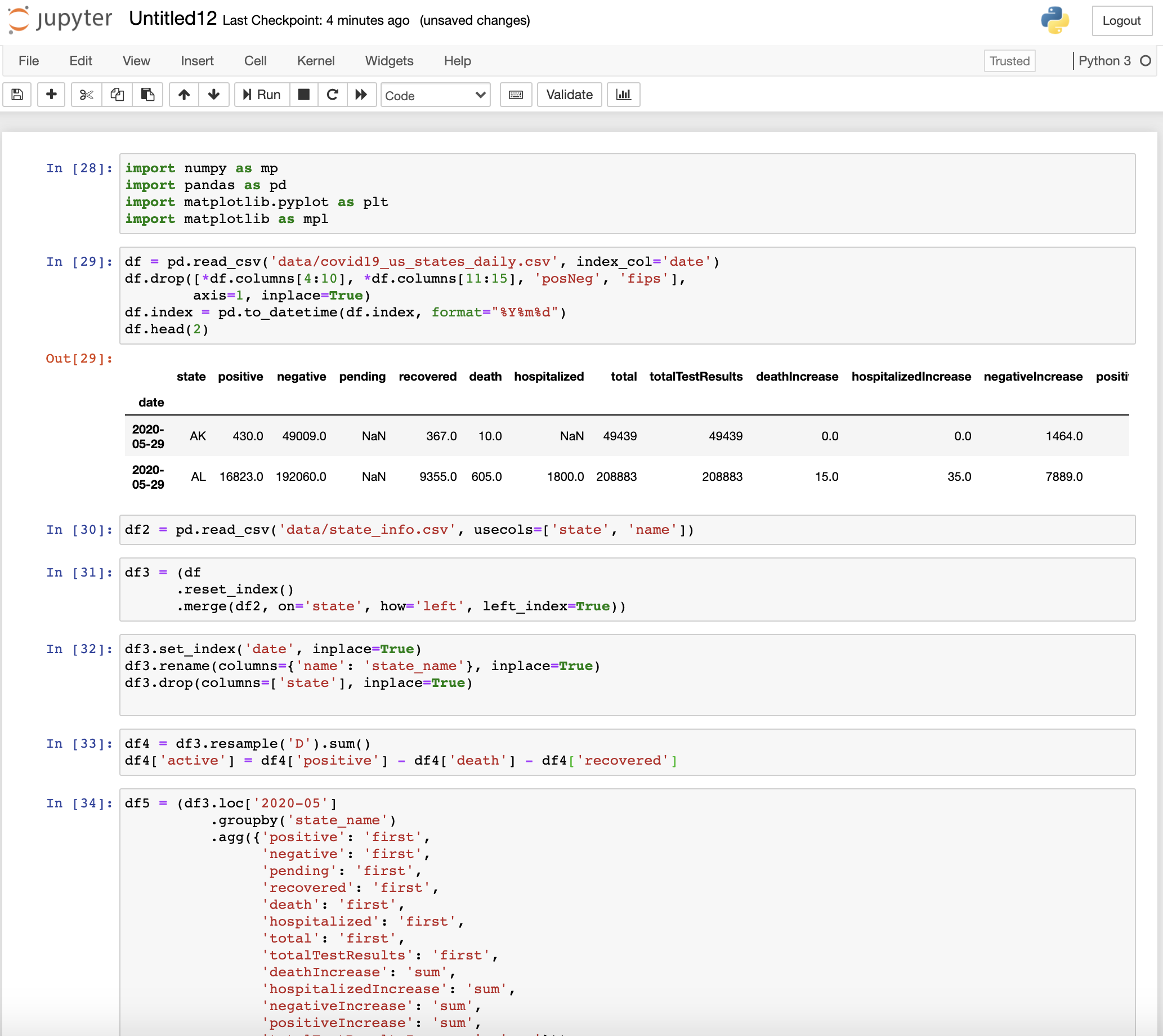
 Does it ring a bell looking at this messy notebook? I am sure you must have created or encountered a similar kind of notebook while performing data analysis tasks in pandas. Pandas is widely used by data scientists and ML Engineers all around the world to perform all kinds of data related tasks like data cleaning and preprocessing, data analysis, data manipulation, data conversion, etc. However, most of us are not using it right, as seen in the above example, which has decreased our productivity a lot. You might wonder then what is the correct way to use pandas. Is there any particular way that we can make the notebook clean and modular so that we can increase our productivity? Luckily, there is a type of quick hack or technique, whatever you may call it, which can be used to greatly improve the workflow and make notebooks not only clean and well organized but highly productive and efficient. The good thing is that you don't need to install any extra packages or libraries. In the end, your notebook will look something like this.  > Note: Dark mode is available on this website. You can switch between the modes by clicking the leftmost button at the bottom of the left sidebar.  # Untitled12.ipynb The way to achieve clean and well-organized pandas notebooks was explored in the presentation [Untitled12.ipynb](https://pydata.org/eindhoven2019/schedule/presentation/19/untitled12ipynb/) by [Vincent D. Warmerdam](https://twitter.com/fishnets88?ref_src=twsrc%5Egoogle%7Ctwcamp%5Eserp%7Ctwgr%5Eauthor) at [PyData Eindhoven 2019](https://pydata.org/eindhoven2019/) The presentation [Untitled12.ipynb: Prevent Miles of Scrolling, Reduce the Spaghetti Code from the Copy Pasta](https://www.youtube.com/watch?v=MpFZUshKypk&t=1292s) has been uploaded in youtube as well. You can watch the video below if you want:
In this article, I will briefly summarize the presentation by [Vincent D. Warmerdam](https://twitter.com/fishnets88?ref_src=twsrc%5Egoogle%7Ctwcamp%5Eserp%7Ctwgr%5Eauthor) and then move on to the code implementation (solution) and a few code examples based on the methods used in his presentation. **The Untitled phenomena** 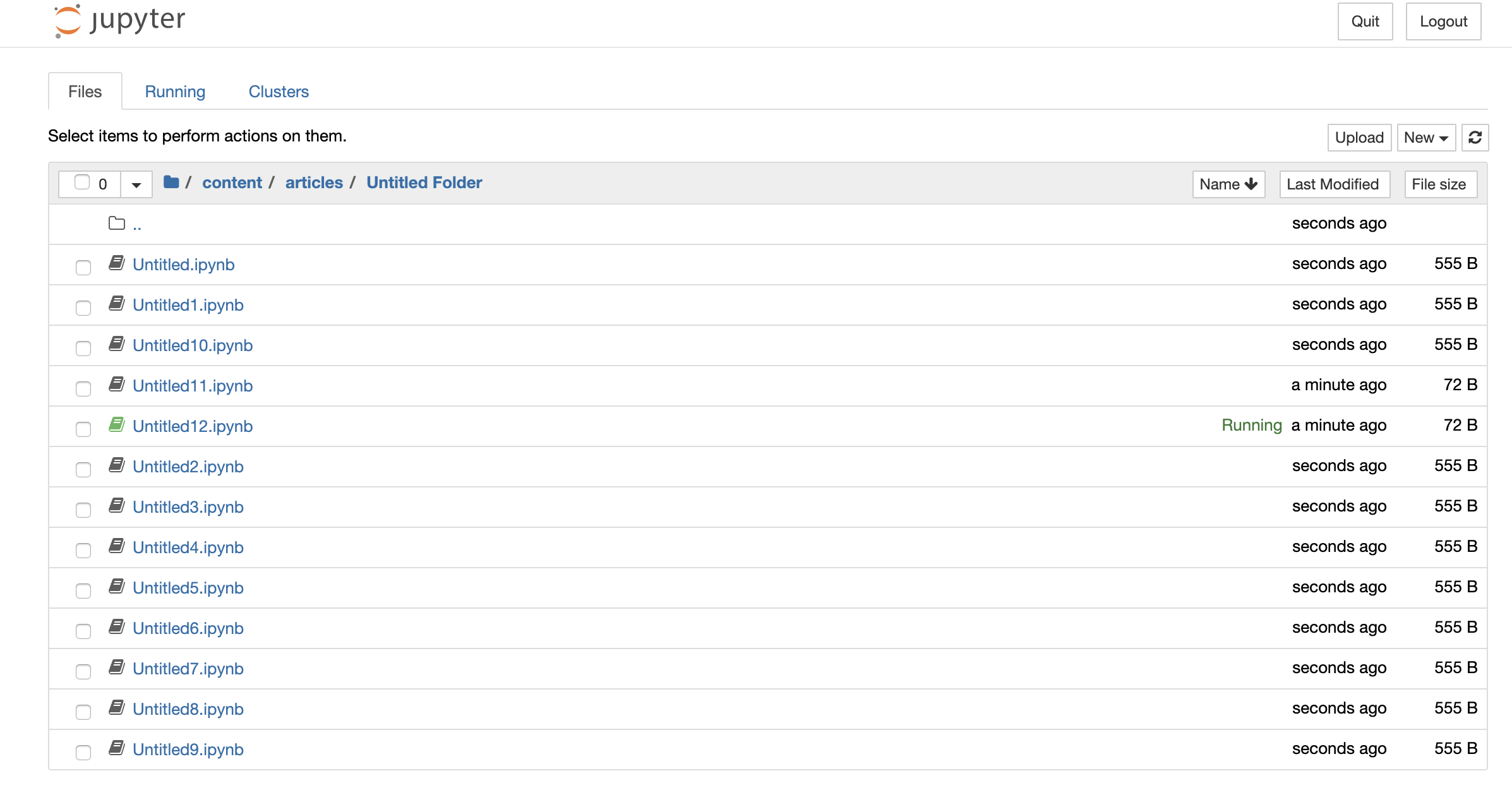 He began his talk by introducing a term called **`Untitled phenomena`**. The term simply refers to the bad practice of not naming the notebook files which eventually creates an unorganized bunch of Untitled notebooks. As a result, he also named the presentation **`Untitled12.ipynb`**. Moreover, not only the bad practice of naming that we follow but also the bad organization of code inside the notebook needs to be improved. Copying and pasting code multiple times creates spaghetti code. This is especially true for a lot of data science based Jupyter notebooks. The goal of his talk was to uncover a great pattern for pandas that would prevent loads of scrolling such that the code behaves like lego. He also gave some useful tricks and tips on how to prevent miles of scrolling and reduce the spaghetti code when creating Jupyter notebooks. ## > [**Skip to coding solution**](#solution) I have initially written a summary of the talk Untitled12.ipynb and explored some common problems in the usual coding style before moving to the solution. If you want to directly jump to the coding solution to create a clean pandas notebook using a pipeline, then click the link above. However, I recommend you to read the common problems I have mentioned before going to the solution. # Contents I will be talking about the following topics which will more or less revolve around his talk. - [Importance of Workflow](#importance) - [The Usual coding style](#current) - [Problems in the usual coding style](#problems) - [Coding Solution](#solution) - [Advantages](#advantages) ## Importance of Workflow At the beginning of the presentation, he began by discussing the following points that highlight the importance of workflows and the need of jupyter-notebook and pandas over excel: - We want to separate the data from the analysis: Tha analysis portion should not modify the raw data. The raw data should be safe from these modifications so that it can be reused later as well. However, this is not possible in excel. - We want to be able to automate our analysis. The main aim of programming and workflow is automation. Our tasks become a lot easier if we can automate the analysis using a pandas script rather than performing the analysis every time using Excel. - We want our analysis to be reproducible i.e. we must be able to reproduce the same analysis results on the data at a later time in the future. - We should not pay a third part obscene amounts of money for something as basic as arithmetic. This budget is better allocated towards innovation and education of staff. However, the current style of coding in pandas and jupyter notebook has solved only the last point. ## The usual coding style Let's explore the common practice of writing pandas code and try to point out the major problems in such approaches. Initially, I will show the general workflow that most of us follow while using pandas. I will be performing some analysis on the real COVID 19 dataset of the U.S. states obtained from [The COVID Tracking Project](https://covidtracking.com/) which is available under the [Creative Commons CC BY-NC-4.0 license](https://creativecommons.org/licenses/by-nc/4.0/). The dataset is updated each day between 4 pm and 5 pm EDT. After showing the common approach, I will point out the major pitfalls and then move on to the solution. First, I will download the U.S. COVID-19 dataset using the API provided by [The COVID Tracking Project](https://covidtracking.com/) ```python !mkdir data !wget -O data/covid19_us_states_daily.csv https://covidtracking.com/api/v1/states/daily.csv !wget -O data/state_info.csv https://covidtracking.com/api/v1/states/info.csv ``` --2020-06-05 16:34:10-- https://covidtracking.com/api/v1/states/daily.csv Resolving covidtracking.com (covidtracking.com)... 104.248.63.231, 2604:a880:400:d1::888:7001 Connecting to covidtracking.com (covidtracking.com)|104.248.63.231|:443... connected. HTTP request sent, awaiting response... 200 OK Length: unspecified [text/csv] Saving to: ‘data/covid19_us_states_daily.csv’ data/covid19_us_sta [ <=> ] 987.40K 3.11MB/s in 0.3s 2020-06-05 16:34:11 (3.11 MB/s) - ‘data/covid19_us_states_daily.csv’ saved [1011093] --2020-06-05 16:34:12-- https://covidtracking.com/api/v1/states/info.csv Resolving covidtracking.com (covidtracking.com)... 104.248.50.87, 2604:a880:400:d1::888:7001 Connecting to covidtracking.com (covidtracking.com)|104.248.50.87|:443... connected. HTTP request sent, awaiting response... 200 OK Length: unspecified [text/csv] Saving to: ‘data/state_info.csv’ data/state_info.csv [ <=> ] 27.67K --.-KB/s in 0.02s 2020-06-05 16:34:13 (1.43 MB/s) - ‘data/state_info.csv’ saved [28329] ```python import pandas as pd # Importing plotly library for plotting interactive graphs import plotly.graph_objects as go from plotly.subplots import make_subplots import plotly.express as px import chart_studio import chart_studio.plotly as py ``` The first step is generally to read or import the data ```python df = pd.read_csv('data/covid19_us_states_daily.csv', index_col='date') df.head() ```
state
positive
negative
pending
hospitalizedCurrently
hospitalizedCumulative
inIcuCurrently
inIcuCumulative
onVentilatorCurrently
onVentilatorCumulative
recovered
dataQualityGrade
lastUpdateEt
dateModified
checkTimeEt
death
hospitalized
dateChecked
fips
positiveIncrease
negativeIncrease
total
totalTestResults
totalTestResultsIncrease
posNeg
deathIncrease
hospitalizedIncrease
hash
commercialScore
negativeRegularScore
negativeScore
positiveScore
score
grade
date
20200604
AK
513.0
59584.0
NaN
13.0
NaN
NaN
NaN
1.0
NaN
376.0
A
6/4/2020 00:00
2020-06-04T00:00:00Z
06/03 20:00
10.0
NaN
2020-06-04T00:00:00Z
2
8
1907
60097
60097
1915
60097
0
0
c1046011af7271cbe2e6698526714c6cb5b92748
0
0
0
0
0
NaN
20200604
AL
19072.0
216227.0
NaN
NaN
1929.0
NaN
601.0
NaN
357.0
11395.0
B
6/4/2020 00:00
2020-06-04T00:00:00Z
06/03 20:00
653.0
1929.0
2020-06-04T00:00:00Z
1
221
3484
235299
235299
3705
235299
0
29
bcbefdb36212ba2b97b5a354f4e45bf16648ee23
0
0
0
0
0
NaN
20200604
AR
8067.0
134413.0
NaN
138.0
757.0
NaN
NaN
30.0
127.0
5717.0
A
6/4/2020 00:00
2020-06-04T00:00:00Z
06/03 20:00
142.0
757.0
2020-06-04T00:00:00Z
5
0
0
142480
142480
0
142480
0
26
acd3a4fbbc3dbb32138725f91e3261d683e7052a
0
0
0
0
0
NaN
20200604
AS
0.0
174.0
NaN
NaN
NaN
NaN
NaN
NaN
NaN
NaN
C
6/1/2020 00:00
2020-06-01T00:00:00Z
05/31 20:00
0.0
NaN
2020-06-01T00:00:00Z
60
0
0
174
174
0
174
0
0
8bbc72fa42781e0549e2e4f9f4c3e7cbef14ab32
0
0
0
0
0
NaN
20200604
AZ
22753.0
227002.0
NaN
1079.0
3195.0
375.0
NaN
223.0
NaN
5172.0
A+
6/4/2020 00:00
2020-06-04T00:00:00Z
06/03 20:00
996.0
3195.0
2020-06-04T00:00:00Z
4
520
4710
249755
249755
5230
249755
15
66
1fa237b8204cd23701577aef6338d339daa4452e
0
0
0
0
0
NaN
After taking a glance at the data, I realize that the date is not formatted well, so I format it. ```python df.index = pd.to_datetime(df.index, format="%Y%m%d") df.head() ```
state
positive
negative
pending
hospitalizedCurrently
hospitalizedCumulative
inIcuCurrently
inIcuCumulative
onVentilatorCurrently
onVentilatorCumulative
recovered
dataQualityGrade
lastUpdateEt
dateModified
checkTimeEt
death
hospitalized
dateChecked
fips
positiveIncrease
negativeIncrease
total
totalTestResults
totalTestResultsIncrease
posNeg
deathIncrease
hospitalizedIncrease
hash
commercialScore
negativeRegularScore
negativeScore
positiveScore
score
grade
date
2020-06-04
AK
513.0
59584.0
NaN
13.0
NaN
NaN
NaN
1.0
NaN
376.0
A
6/4/2020 00:00
2020-06-04T00:00:00Z
06/03 20:00
10.0
NaN
2020-06-04T00:00:00Z
2
8
1907
60097
60097
1915
60097
0
0
c1046011af7271cbe2e6698526714c6cb5b92748
0
0
0
0
0
NaN
2020-06-04
AL
19072.0
216227.0
NaN
NaN
1929.0
NaN
601.0
NaN
357.0
11395.0
B
6/4/2020 00:00
2020-06-04T00:00:00Z
06/03 20:00
653.0
1929.0
2020-06-04T00:00:00Z
1
221
3484
235299
235299
3705
235299
0
29
bcbefdb36212ba2b97b5a354f4e45bf16648ee23
0
0
0
0
0
NaN
2020-06-04
AR
8067.0
134413.0
NaN
138.0
757.0
NaN
NaN
30.0
127.0
5717.0
A
6/4/2020 00:00
2020-06-04T00:00:00Z
06/03 20:00
142.0
757.0
2020-06-04T00:00:00Z
5
0
0
142480
142480
0
142480
0
26
acd3a4fbbc3dbb32138725f91e3261d683e7052a
0
0
0
0
0
NaN
2020-06-04
AS
0.0
174.0
NaN
NaN
NaN
NaN
NaN
NaN
NaN
NaN
C
6/1/2020 00:00
2020-06-01T00:00:00Z
05/31 20:00
0.0
NaN
2020-06-01T00:00:00Z
60
0
0
174
174
0
174
0
0
8bbc72fa42781e0549e2e4f9f4c3e7cbef14ab32
0
0
0
0
0
NaN
2020-06-04
AZ
22753.0
227002.0
NaN
1079.0
3195.0
375.0
NaN
223.0
NaN
5172.0
A+
6/4/2020 00:00
2020-06-04T00:00:00Z
06/03 20:00
996.0
3195.0
2020-06-04T00:00:00Z
4
520
4710
249755
249755
5230
249755
15
66
1fa237b8204cd23701577aef6338d339daa4452e
0
0
0
0
0
NaN
Then, I try to view some additional information about the dataset ```python df.info() ``` DatetimeIndex: 5113 entries, 2020-06-04 to 2020-01-22 Data columns (total 34 columns): # Column Non-Null Count Dtype --- ------ -------------- ----- 0 state 5113 non-null object 1 positive 5098 non-null float64 2 negative 4902 non-null float64 3 pending 842 non-null float64 4 hospitalizedCurrently 2591 non-null float64 5 hospitalizedCumulative 2318 non-null float64 6 inIcuCurrently 1362 non-null float64 7 inIcuCumulative 576 non-null float64 8 onVentilatorCurrently 1157 non-null float64 9 onVentilatorCumulative 198 non-null float64 10 recovered 2409 non-null float64 11 dataQualityGrade 4012 non-null object 12 lastUpdateEt 4758 non-null object 13 dateModified 4758 non-null object 14 checkTimeEt 4758 non-null object 15 death 4388 non-null float64 16 hospitalized 2318 non-null float64 17 dateChecked 4758 non-null object 18 fips 5113 non-null int64 19 positiveIncrease 5113 non-null int64 20 negativeIncrease 5113 non-null int64 21 total 5113 non-null int64 22 totalTestResults 5113 non-null int64 23 totalTestResultsIncrease 5113 non-null int64 24 posNeg 5113 non-null int64 25 deathIncrease 5113 non-null int64 26 hospitalizedIncrease 5113 non-null int64 27 hash 5113 non-null object 28 commercialScore 5113 non-null int64 29 negativeRegularScore 5113 non-null int64 30 negativeScore 5113 non-null int64 31 positiveScore 5113 non-null int64 32 score 5113 non-null int64 33 grade 0 non-null float64 dtypes: float64(13), int64(14), object(7) memory usage: 1.4+ MB You can see that various columns are not of use. So, I decide to remove such columns. ```python df.drop([*df.columns[4:10], *df.columns[11:15], 'posNeg', 'fips'], axis=1, inplace=True) df.info() ``` DatetimeIndex: 5113 entries, 2020-06-04 to 2020-01-22 Data columns (total 22 columns): # Column Non-Null Count Dtype --- ------ -------------- ----- 0 state 5113 non-null object 1 positive 5098 non-null float64 2 negative 4902 non-null float64 3 pending 842 non-null float64 4 recovered 2409 non-null float64 5 death 4388 non-null float64 6 hospitalized 2318 non-null float64 7 dateChecked 4758 non-null object 8 positiveIncrease 5113 non-null int64 9 negativeIncrease 5113 non-null int64 10 total 5113 non-null int64 11 totalTestResults 5113 non-null int64 12 totalTestResultsIncrease 5113 non-null int64 13 deathIncrease 5113 non-null int64 14 hospitalizedIncrease 5113 non-null int64 15 hash 5113 non-null object 16 commercialScore 5113 non-null int64 17 negativeRegularScore 5113 non-null int64 18 negativeScore 5113 non-null int64 19 positiveScore 5113 non-null int64 20 score 5113 non-null int64 21 grade 0 non-null float64 dtypes: float64(7), int64(12), object(3) memory usage: 918.7+ KB I also realize that there are a lot of missing (nan or null) values. So, I replace the missing values by 0. ```python df.fillna(value=0, inplace=True) df.head() ```
state
positive
negative
pending
recovered
death
hospitalized
dateChecked
positiveIncrease
negativeIncrease
total
totalTestResults
totalTestResultsIncrease
deathIncrease
hospitalizedIncrease
hash
commercialScore
negativeRegularScore
negativeScore
positiveScore
score
grade
date
2020-06-04
AK
513.0
59584.0
0.0
376.0
10.0
0.0
2020-06-04T00:00:00Z
8
1907
60097
60097
1915
0
0
c1046011af7271cbe2e6698526714c6cb5b92748
0
0
0
0
0
0.0
2020-06-04
AL
19072.0
216227.0
0.0
11395.0
653.0
1929.0
2020-06-04T00:00:00Z
221
3484
235299
235299
3705
0
29
bcbefdb36212ba2b97b5a354f4e45bf16648ee23
0
0
0
0
0
0.0
2020-06-04
AR
8067.0
134413.0
0.0
5717.0
142.0
757.0
2020-06-04T00:00:00Z
0
0
142480
142480
0
0
26
acd3a4fbbc3dbb32138725f91e3261d683e7052a
0
0
0
0
0
0.0
2020-06-04
AS
0.0
174.0
0.0
0.0
0.0
0.0
2020-06-01T00:00:00Z
0
0
174
174
0
0
0
8bbc72fa42781e0549e2e4f9f4c3e7cbef14ab32
0
0
0
0
0
0.0
2020-06-04
AZ
22753.0
227002.0
0.0
5172.0
996.0
3195.0
2020-06-04T00:00:00Z
520
4710
249755
249755
5230
15
66
1fa237b8204cd23701577aef6338d339daa4452e
0
0
0
0
0
0.0
I also want to add a column corresponding to the state name instead of the abbreviation. So, I merge state_info with the current dataframe. ```python df2 = pd.read_csv('data/state_info.csv', usecols=['state', 'name']) df3 = (df .reset_index() .merge(df2, on='state', how='left', left_index=True)) df3.head() ```
date
state
positive
negative
pending
recovered
death
hospitalized
dateChecked
positiveIncrease
negativeIncrease
total
totalTestResults
totalTestResultsIncrease
deathIncrease
hospitalizedIncrease
hash
commercialScore
negativeRegularScore
negativeScore
positiveScore
score
grade
name
0
2020-06-04
AK
513.0
59584.0
0.0
376.0
10.0
0.0
2020-06-04T00:00:00Z
8
1907
60097
60097
1915
0
0
c1046011af7271cbe2e6698526714c6cb5b92748
0
0
0
0
0
0.0
Alaska
1
2020-06-04
AL
19072.0
216227.0
0.0
11395.0
653.0
1929.0
2020-06-04T00:00:00Z
221
3484
235299
235299
3705
0
29
bcbefdb36212ba2b97b5a354f4e45bf16648ee23
0
0
0
0
0
0.0
Alabama
2
2020-06-04
AR
8067.0
134413.0
0.0
5717.0
142.0
757.0
2020-06-04T00:00:00Z
0
0
142480
142480
0
0
26
acd3a4fbbc3dbb32138725f91e3261d683e7052a
0
0
0
0
0
0.0
Arkansas
3
2020-06-04
AS
0.0
174.0
0.0
0.0
0.0
0.0
2020-06-01T00:00:00Z
0
0
174
174
0
0
0
8bbc72fa42781e0549e2e4f9f4c3e7cbef14ab32
0
0
0
0
0
0.0
American Samoa
4
2020-06-04
AZ
22753.0
227002.0
0.0
5172.0
996.0
3195.0
2020-06-04T00:00:00Z
520
4710
249755
249755
5230
15
66
1fa237b8204cd23701577aef6338d339daa4452e
0
0
0
0
0
0.0
Arizona
I realize that the date index is lost. So, I reset the date index. Also, it is better to rename the column name as state_name. ```python df3.set_index('date', inplace=True) df3.rename(columns={'name': 'state_name'}, inplace=True) df3.head() ```
state
positive
negative
pending
recovered
death
hospitalized
dateChecked
positiveIncrease
negativeIncrease
total
totalTestResults
totalTestResultsIncrease
deathIncrease
hospitalizedIncrease
hash
commercialScore
negativeRegularScore
negativeScore
positiveScore
score
grade
state_name
date
2020-06-04
AK
513.0
59584.0
0.0
376.0
10.0
0.0
2020-06-04T00:00:00Z
8
1907
60097
60097
1915
0
0
c1046011af7271cbe2e6698526714c6cb5b92748
0
0
0
0
0
0.0
Alaska
2020-06-04
AL
19072.0
216227.0
0.0
11395.0
653.0
1929.0
2020-06-04T00:00:00Z
221
3484
235299
235299
3705
0
29
bcbefdb36212ba2b97b5a354f4e45bf16648ee23
0
0
0
0
0
0.0
Alabama
2020-06-04
AR
8067.0
134413.0
0.0
5717.0
142.0
757.0
2020-06-04T00:00:00Z
0
0
142480
142480
0
0
26
acd3a4fbbc3dbb32138725f91e3261d683e7052a
0
0
0
0
0
0.0
Arkansas
2020-06-04
AS
0.0
174.0
0.0
0.0
0.0
0.0
2020-06-01T00:00:00Z
0
0
174
174
0
0
0
8bbc72fa42781e0549e2e4f9f4c3e7cbef14ab32
0
0
0
0
0
0.0
American Samoa
2020-06-04
AZ
22753.0
227002.0
0.0
5172.0
996.0
3195.0
2020-06-04T00:00:00Z
520
4710
249755
249755
5230
15
66
1fa237b8204cd23701577aef6338d339daa4452e
0
0
0
0
0
0.0
Arizona
Now that the data is ready for some analysis, I decide to plot deaths count in each state indexed by date using the interactive [plotly library](https://plotly.com/). ```python fig1 = px.line(df3, x=df3.index, y='death', color='state') fig1.update_layout(xaxis_title='date', title='Total deaths in each state (Cumulative)') py.plot(fig1, filename = 'daily_deaths', auto_open=True) ``` 'https://plotly.com/~ayush.kumar.shah/1/'
> Note: These plots are interactive, so you can zoom in or out, pinch, hover over the graph, download it, and so on. Now, I decide to calculate the total deaths in the US across all states and plot it. ```python df4 = df3.resample('D').sum() df4.head() ```
positive
negative
pending
recovered
death
hospitalized
positiveIncrease
negativeIncrease
total
totalTestResults
totalTestResultsIncrease
deathIncrease
hospitalizedIncrease
commercialScore
negativeRegularScore
negativeScore
positiveScore
score
grade
date
2020-01-22
1.0
0.0
0.0
0.0
0.0
0.0
0
0
1
1
0
0
0
0
0
0
0
0
0.0
2020-01-23
1.0
0.0
0.0
0.0
0.0
0.0
0
0
1
1
0
0
0
0
0
0
0
0
0.0
2020-01-24
1.0
0.0
0.0
0.0
0.0
0.0
0
0
1
1
0
0
0
0
0
0
0
0
0.0
2020-01-25
1.0
0.0
0.0
0.0
0.0
0.0
0
0
1
1
0
0
0
0
0
0
0
0
0.0
2020-01-26
1.0
0.0
0.0
0.0
0.0
0.0
0
0
1
1
0
0
0
0
0
0
0
0
0.0
```python fig2 = px.line(df4, x=df4.index, y='death') fig2.update_layout(xaxis_title='date', title='Total deaths in the U.S. (Cumulative)') py.plot(fig2, filename = 'total_daily_deaths', auto_open=True) ``` 'https://plotly.com/~ayush.kumar.shah/4/'
I also want to calculate the number of Active cases i.e. > Active = positive - deaths - recovered ```python df4['active'] = df4['positive'] - df4['death'] - df4['recovered'] ``` Now, after calculating the active column, I want to plot active cases instead of death. So, I go to the previous cell and replace `death` by `active` and generate the plot. In [25]: df4['~~death~~'].plot() In [25]: df4['active'].plot() ```python fig3 = px.line(df4, x=df4.index, y='active') fig3.update_layout(xaxis_title='date', title='Total active cases in the U.S. (Cumulative)') py.plot(fig3, filename = 'total_daily_active', auto_open=True) ``` 'https://plotly.com/~ayush.kumar.shah/6/'
Then I decide to calculate the statistics of a single month of May only. Since the data is cumulative, I need to subtract the data of May from data of April to find the increase in various statistics in May after which I plot the results. ```python df5 = (df3.loc['2020-05'] .groupby('state_name') .agg({'positive': 'first', 'negative': 'first', 'pending': 'first', 'recovered': 'first', 'death': 'first', 'hospitalized': 'first', 'total': 'first', 'totalTestResults': 'first', 'deathIncrease': 'sum', 'hospitalizedIncrease': 'sum', 'negativeIncrease': 'sum', 'positiveIncrease': 'sum', 'totalTestResultsIncrease': 'sum'})) df6 = (df3.loc['2020-04'] .groupby('state_name') .agg({'positive': 'first', 'negative': 'first', 'pending': 'first', 'recovered': 'first', 'death': 'first', 'hospitalized': 'first', 'total': 'first', 'totalTestResults': 'first', 'deathIncrease': 'sum', 'hospitalizedIncrease': 'sum', 'negativeIncrease': 'sum', 'positiveIncrease': 'sum', 'totalTestResultsIncrease': 'sum'})) df7 = df5.sub(df6) df7.head() ```
positive
negative
pending
recovered
death
hospitalized
total
totalTestResults
deathIncrease
hospitalizedIncrease
negativeIncrease
positiveIncrease
totalTestResultsIncrease
state_name
Alabama
10884.0
119473.0
0.0
9355.0
362.0
866.0
130357
130357
106
-112
45594
4846
50440
Alaska
79.0
32497.0
0.0
116.0
1.0
0.0
32576
32576
-5
7
17327
-157
17170
American Samoa
0.0
171.0
-17.0
0.0
0.0
0.0
154
171
0
0
171
0
171
Arizona
12288.0
141132.0
0.0
3262.0
586.0
1829.0
153420
153420
290
660
95076
5929
101005
Arkansas
3998.0
77138.0
0.0
3970.0
72.0
309.0
81136
81136
19
-93
37973
1266
39239
```python fig4 = px.bar(df7, x=df7.index, y='death') fig4.update_layout(xaxis_title='state_name', title='Total Deaths in th US in May only') py.plot(fig4, filename = 'total_deaths_May', auto_open=True) ``` 'https://plotly.com/~ayush.kumar.shah/12/'
## Problems in the usual coding style Now that I have demonstrated the usual approach followed in pandas notebook, let's discuss the problems in this approach. ### 1. Flow is disrupted: The flow of the notebook is very difficult to understand and also creates problems. For example, we may create a variable name under the plot that needs it. In the above code as well, we created **`df3['active']`** below the cell in which it is needed. So, it may cause errors when run by others. Also, you may have to scroll the notebook for miles and miles. ### 2. No reproducibility: When the notebook is shared with others, the other person faces a lot of problems to execute or understand the notebook. For instance, the name of the dataframes doesn't signify any information about the type of dataframe. It runs from **`df1`** to **`df7`** and creates a lot of confusion. But you want to create a notebook which is very easy to iterate on and the one you can share with your colleagues. ### 3. Difficult to move the code to production: With this approach, your code is not ready to move into production. You end up having to rewrite the whole notebook before moving it to production which is not effective. ### 4. Unable to automate: The notebook in the current condition cannot be automated for analysis since there may occur a lot of problems like an error in code execution, unavailability of filenames used. Although the code may give an interesting conclusion or desired output, we are not quite sure that conclusion is at least correct. Despite having so many problems associated with this approach, it is common for everyone to still use this type of flow while making a notebook since while coding, people enjoy when the code works when they check the outputs and hence keep on similarly continuing the coding. ## Coding Solution ### 1. Naming convention Follow a naming convention for the notebook according to the task as suggested by [Cookiecutter Data Science](https://drivendata.github.io/cookiecutter-data-science/#notebooks-are-for-exploration-and-communication) that shows the owner and the order the analysis was done in. You can use the format **`--.ipynb`** (e.g., **`0.1-ayush-visualize-corona-us.ipynb`**). ### 2. Plan your steps beforehand Load the data and then think in advance about all the steps of analysis or tasks you could be doing in the notebook. You don't need to think the logic right away but just keep in mind the steps. ```python df = pd.read_csv('data/covid19_us_states_daily.csv', index_col='date') ``` ### 3. Create functions You know that initially, you want to clean the data and make sure the columns and indexes are in a proper usable format. So, why not create a function for that and name it according to the subtasks on the dataframe. > For example, initially you want to make the index a proper datetime object. Then you may want to do remove the duplicates, then add state name. Just add these functions without even thinking the logic and then later you can add the logic. This way, you will be on track and not lost. The functions are created after creating the decorator. ### 4. Create proper decorators Before adding functions, let's also think about some additional utility that would be helpful. During the pandas analysis, you often check the shape, columns, and other information associated to the dataframe after performing an operation. However, a decorator can help automate this process. **`Decorator`** is simply a function that expects a function and returns a function. It's really functional right, haha. Don't get confused by the definition. It is not so difficult as it sounds. We will see how it works in the code below. Also, if you are not familiar with decorators or want to learn more about it, you can visit the [article by Geir Arne Hjelle](https://realpython.com/primer-on-python-decorators/#simple-decorators). ```python import datetime as dt def df_info(f): def wrapper(df, *args, **kwargs): tic = dt.datetime.now() result = f(df, *args, **kwargs) toc = dt.datetime.now() print("\n\n{} took {} time\n".format(f.__name__, toc - tic)) print("After applying {}\n".format(f.__name__)) print("Shape of df = {}\n".format(result.shape)) print("Columns of df are {}\n".format(result.columns)) print("Index of df is {}\n".format(result.index)) for i in range(100): print("-", end='') return result return wrapper ``` We have created a decorator called **`df_info`** which displays information like time taken by the function, shape, and columns after applying any function **`f`**. The advantage of using a deorator is that we get logging. You can modify the decorator according to the information that you want to log or display after performing an operation on the dataframe. Now, we create functions as our plan and use these decorators on them by using **`@df_info`**. This will be equivalent to calling **`df_info(f(df, *args, **kwargs))`** ```python @df_info def create_dateindex(df): df.index = pd.to_datetime(df.index, format="%Y%m%d") return df @df_info def remove_columns(df): df.drop([*df.columns[4:10], *df.columns[11:15], 'posNeg', 'fips'], axis=1, inplace=True) return df @df_info def fill_missing(df): df.fillna(value=0, inplace=True) return df @df_info def add_state_name(df): _df = pd.read_csv('data/state_info.csv', usecols=['state', 'name']) df = (df .reset_index() .merge(_df, on='state', how='left', left_index=True)) df.set_index('date', inplace=True) df.rename(columns={'name': 'state_name'}, inplace=True) return df @df_info def drop_state(df): df.drop(columns=['state'], inplace=True) return df @df_info def sample_daily(df): df = df.resample('D').sum() return df @df_info def add_active_cases(df): df['active'] = df['positive'] - df['death'] - df['recovered'] return df def aggregate_monthly(df, month): df = (df.loc[month] .groupby('state_name') .agg({'positive': 'first', 'negative': 'first', 'pending': 'first', 'recovered': 'first', 'death': 'first', 'hospitalized': 'first', 'total': 'first', 'totalTestResults': 'first', 'deathIncrease': 'sum', 'hospitalizedIncrease': 'sum', 'negativeIncrease': 'sum', 'positiveIncrease': 'sum', 'totalTestResultsIncrease': 'sum'})) return df @df_info def create_month_only(df, month): df_current = aggregate_monthly(df, month) if int(month[-2:]) == 0: prev_month = str(int(month[:4]) - 1) + '-12' else: prev_month = month[:5] + '{:02d}'.format(int(month[-2:])-1) df_previous = aggregate_monthly(df, prev_month) df = df_current.sub(df_previous) return df ``` ### 5. Remove side effect However, these functions make changes that are inplace (side effects) i.e. modifies the originally loaded dataframe. So, to solve this, we add a function called start pipeline, which returns a copy of dataframe. ```python def start_pipeline(df): return df.copy() ``` ### 6. Constructing pandas pipelines (Main step) Now, let's use these functions to achieve the previous tasks using **`pipe`** ```python df_daily = (df.pipe(start_pipeline) .pipe(create_dateindex) .pipe(remove_columns) .pipe(fill_missing) .pipe(add_state_name) .pipe(sample_daily) .pipe(add_active_cases)) ``` create_dateindex took 0:00:00.003388 time After applying create_dateindex Shape of df = (5113, 34) Columns of df are Index(['state', 'positive', 'negative', 'pending', 'hospitalizedCurrently', 'hospitalizedCumulative', 'inIcuCurrently', 'inIcuCumulative', 'onVentilatorCurrently', 'onVentilatorCumulative', 'recovered', 'dataQualityGrade', 'lastUpdateEt', 'dateModified', 'checkTimeEt', 'death', 'hospitalized', 'dateChecked', 'fips', 'positiveIncrease', 'negativeIncrease', 'total', 'totalTestResults', 'totalTestResultsIncrease', 'posNeg', 'deathIncrease', 'hospitalizedIncrease', 'hash', 'commercialScore', 'negativeRegularScore', 'negativeScore', 'positiveScore', 'score', 'grade'], dtype='object') Index of df is DatetimeIndex(['2020-06-04', '2020-06-04', '2020-06-04', '2020-06-04', '2020-06-04', '2020-06-04', '2020-06-04', '2020-06-04', '2020-06-04', '2020-06-04', ... '2020-01-31', '2020-01-30', '2020-01-29', '2020-01-28', '2020-01-27', '2020-01-26', '2020-01-25', '2020-01-24', '2020-01-23', '2020-01-22'], dtype='datetime64[ns]', name='date', length=5113, freq=None) ---------------------------------------------------------------------------------------------------- remove_columns took 0:00:00.002087 time After applying remove_columns Shape of df = (5113, 22) Columns of df are Index(['state', 'positive', 'negative', 'pending', 'recovered', 'death', 'hospitalized', 'dateChecked', 'positiveIncrease', 'negativeIncrease', 'total', 'totalTestResults', 'totalTestResultsIncrease', 'deathIncrease', 'hospitalizedIncrease', 'hash', 'commercialScore', 'negativeRegularScore', 'negativeScore', 'positiveScore', 'score', 'grade'], dtype='object') Index of df is DatetimeIndex(['2020-06-04', '2020-06-04', '2020-06-04', '2020-06-04', '2020-06-04', '2020-06-04', '2020-06-04', '2020-06-04', '2020-06-04', '2020-06-04', ... '2020-01-31', '2020-01-30', '2020-01-29', '2020-01-28', '2020-01-27', '2020-01-26', '2020-01-25', '2020-01-24', '2020-01-23', '2020-01-22'], dtype='datetime64[ns]', name='date', length=5113, freq=None) ---------------------------------------------------------------------------------------------------- fill_missing took 0:00:00.006381 time After applying fill_missing Shape of df = (5113, 22) Columns of df are Index(['state', 'positive', 'negative', 'pending', 'recovered', 'death', 'hospitalized', 'dateChecked', 'positiveIncrease', 'negativeIncrease', 'total', 'totalTestResults', 'totalTestResultsIncrease', 'deathIncrease', 'hospitalizedIncrease', 'hash', 'commercialScore', 'negativeRegularScore', 'negativeScore', 'positiveScore', 'score', 'grade'], dtype='object') Index of df is DatetimeIndex(['2020-06-04', '2020-06-04', '2020-06-04', '2020-06-04', '2020-06-04', '2020-06-04', '2020-06-04', '2020-06-04', '2020-06-04', '2020-06-04', ... '2020-01-31', '2020-01-30', '2020-01-29', '2020-01-28', '2020-01-27', '2020-01-26', '2020-01-25', '2020-01-24', '2020-01-23', '2020-01-22'], dtype='datetime64[ns]', name='date', length=5113, freq=None) ---------------------------------------------------------------------------------------------------- add_state_name took 0:00:00.015122 time After applying add_state_name Shape of df = (5113, 23) Columns of df are Index(['state', 'positive', 'negative', 'pending', 'recovered', 'death', 'hospitalized', 'dateChecked', 'positiveIncrease', 'negativeIncrease', 'total', 'totalTestResults', 'totalTestResultsIncrease', 'deathIncrease', 'hospitalizedIncrease', 'hash', 'commercialScore', 'negativeRegularScore', 'negativeScore', 'positiveScore', 'score', 'grade', 'state_name'], dtype='object') Index of df is DatetimeIndex(['2020-06-04', '2020-06-04', '2020-06-04', '2020-06-04', '2020-06-04', '2020-06-04', '2020-06-04', '2020-06-04', '2020-06-04', '2020-06-04', ... '2020-01-31', '2020-01-30', '2020-01-29', '2020-01-28', '2020-01-27', '2020-01-26', '2020-01-25', '2020-01-24', '2020-01-23', '2020-01-22'], dtype='datetime64[ns]', name='date', length=5113, freq=None) ---------------------------------------------------------------------------------------------------- sample_daily took 0:00:00.017170 time After applying sample_daily Shape of df = (135, 19) Columns of df are Index(['positive', 'negative', 'pending', 'recovered', 'death', 'hospitalized', 'positiveIncrease', 'negativeIncrease', 'total', 'totalTestResults', 'totalTestResultsIncrease', 'deathIncrease', 'hospitalizedIncrease', 'commercialScore', 'negativeRegularScore', 'negativeScore', 'positiveScore', 'score', 'grade'], dtype='object') Index of df is DatetimeIndex(['2020-01-22', '2020-01-23', '2020-01-24', '2020-01-25', '2020-01-26', '2020-01-27', '2020-01-28', '2020-01-29', '2020-01-30', '2020-01-31', ... '2020-05-26', '2020-05-27', '2020-05-28', '2020-05-29', '2020-05-30', '2020-05-31', '2020-06-01', '2020-06-02', '2020-06-03', '2020-06-04'], dtype='datetime64[ns]', name='date', length=135, freq='D') ---------------------------------------------------------------------------------------------------- add_active_cases took 0:00:00.002020 time After applying add_active_cases Shape of df = (135, 20) Columns of df are Index(['positive', 'negative', 'pending', 'recovered', 'death', 'hospitalized', 'positiveIncrease', 'negativeIncrease', 'total', 'totalTestResults', 'totalTestResultsIncrease', 'deathIncrease', 'hospitalizedIncrease', 'commercialScore', 'negativeRegularScore', 'negativeScore', 'positiveScore', 'score', 'grade', 'active'], dtype='object') Index of df is DatetimeIndex(['2020-01-22', '2020-01-23', '2020-01-24', '2020-01-25', '2020-01-26', '2020-01-27', '2020-01-28', '2020-01-29', '2020-01-30', '2020-01-31', ... '2020-05-26', '2020-05-27', '2020-05-28', '2020-05-29', '2020-05-30', '2020-05-31', '2020-06-01', '2020-06-02', '2020-06-03', '2020-06-04'], dtype='datetime64[ns]', name='date', length=135, freq='D') Check out all the logs displayed above. We are able to view in detail how each operation changed the data without having to print the dataframe after each operation. ```python fig2 = px.line(df_daily, x=df_daily.index, y='death') fig2.update_layout(xaxis_title='date', title='Total deaths in the U.S. (Cumulative)') py.plot(fig2, filename = 'total_daily_deaths', auto_open=True) ``` 'https://plotly.com/~ayush.kumar.shah/4/'
```python fig3 = px.line(df_daily, x=df_daily.index, y='active') fig3.update_layout(xaxis_title='date', title='Total active cases in the U.S. (Cumulative)') py.plot(fig3, filename = 'total_daily_active', auto_open=True) ``` 'https://plotly.com/~ayush.kumar.shah/6/'
```python df_may = create_month_only( df=(df.pipe(start_pipeline) .pipe(create_dateindex) .pipe(remove_columns) .pipe(fill_missing) .pipe(add_state_name)), month='2020-05') ``` create_dateindex took 0:00:00.002492 time After applying create_dateindex Shape of df = (5113, 34) Columns of df are Index(['state', 'positive', 'negative', 'pending', 'hospitalizedCurrently', 'hospitalizedCumulative', 'inIcuCurrently', 'inIcuCumulative', 'onVentilatorCurrently', 'onVentilatorCumulative', 'recovered', 'dataQualityGrade', 'lastUpdateEt', 'dateModified', 'checkTimeEt', 'death', 'hospitalized', 'dateChecked', 'fips', 'positiveIncrease', 'negativeIncrease', 'total', 'totalTestResults', 'totalTestResultsIncrease', 'posNeg', 'deathIncrease', 'hospitalizedIncrease', 'hash', 'commercialScore', 'negativeRegularScore', 'negativeScore', 'positiveScore', 'score', 'grade'], dtype='object') Index of df is DatetimeIndex(['2020-06-04', '2020-06-04', '2020-06-04', '2020-06-04', '2020-06-04', '2020-06-04', '2020-06-04', '2020-06-04', '2020-06-04', '2020-06-04', ... '2020-01-31', '2020-01-30', '2020-01-29', '2020-01-28', '2020-01-27', '2020-01-26', '2020-01-25', '2020-01-24', '2020-01-23', '2020-01-22'], dtype='datetime64[ns]', name='date', length=5113, freq=None) ---------------------------------------------------------------------------------------------------- remove_columns took 0:00:00.002219 time After applying remove_columns Shape of df = (5113, 22) Columns of df are Index(['state', 'positive', 'negative', 'pending', 'recovered', 'death', 'hospitalized', 'dateChecked', 'positiveIncrease', 'negativeIncrease', 'total', 'totalTestResults', 'totalTestResultsIncrease', 'deathIncrease', 'hospitalizedIncrease', 'hash', 'commercialScore', 'negativeRegularScore', 'negativeScore', 'positiveScore', 'score', 'grade'], dtype='object') Index of df is DatetimeIndex(['2020-06-04', '2020-06-04', '2020-06-04', '2020-06-04', '2020-06-04', '2020-06-04', '2020-06-04', '2020-06-04', '2020-06-04', '2020-06-04', ... '2020-01-31', '2020-01-30', '2020-01-29', '2020-01-28', '2020-01-27', '2020-01-26', '2020-01-25', '2020-01-24', '2020-01-23', '2020-01-22'], dtype='datetime64[ns]', name='date', length=5113, freq=None) ---------------------------------------------------------------------------------------------------- fill_missing took 0:00:00.001883 time After applying fill_missing Shape of df = (5113, 22) Columns of df are Index(['state', 'positive', 'negative', 'pending', 'recovered', 'death', 'hospitalized', 'dateChecked', 'positiveIncrease', 'negativeIncrease', 'total', 'totalTestResults', 'totalTestResultsIncrease', 'deathIncrease', 'hospitalizedIncrease', 'hash', 'commercialScore', 'negativeRegularScore', 'negativeScore', 'positiveScore', 'score', 'grade'], dtype='object') Index of df is DatetimeIndex(['2020-06-04', '2020-06-04', '2020-06-04', '2020-06-04', '2020-06-04', '2020-06-04', '2020-06-04', '2020-06-04', '2020-06-04', '2020-06-04', ... '2020-01-31', '2020-01-30', '2020-01-29', '2020-01-28', '2020-01-27', '2020-01-26', '2020-01-25', '2020-01-24', '2020-01-23', '2020-01-22'], dtype='datetime64[ns]', name='date', length=5113, freq=None) ---------------------------------------------------------------------------------------------------- add_state_name took 0:00:00.014981 time After applying add_state_name Shape of df = (5113, 23) Columns of df are Index(['state', 'positive', 'negative', 'pending', 'recovered', 'death', 'hospitalized', 'dateChecked', 'positiveIncrease', 'negativeIncrease', 'total', 'totalTestResults', 'totalTestResultsIncrease', 'deathIncrease', 'hospitalizedIncrease', 'hash', 'commercialScore', 'negativeRegularScore', 'negativeScore', 'positiveScore', 'score', 'grade', 'state_name'], dtype='object') Index of df is DatetimeIndex(['2020-06-04', '2020-06-04', '2020-06-04', '2020-06-04', '2020-06-04', '2020-06-04', '2020-06-04', '2020-06-04', '2020-06-04', '2020-06-04', ... '2020-01-31', '2020-01-30', '2020-01-29', '2020-01-28', '2020-01-27', '2020-01-26', '2020-01-25', '2020-01-24', '2020-01-23', '2020-01-22'], dtype='datetime64[ns]', name='date', length=5113, freq=None) ---------------------------------------------------------------------------------------------------- create_month_only took 0:00:00.031071 time After applying create_month_only Shape of df = (56, 13) Columns of df are Index(['positive', 'negative', 'pending', 'recovered', 'death', 'hospitalized', 'total', 'totalTestResults', 'deathIncrease', 'hospitalizedIncrease', 'negativeIncrease', 'positiveIncrease', 'totalTestResultsIncrease'], dtype='object') Index of df is Index(['Alabama', 'Alaska', 'American Samoa', 'Arizona', 'Arkansas', 'California', 'Colorado', 'Connecticut', 'Delaware', 'District Of Columbia', 'Florida', 'Georgia', 'Guam', 'Hawaii', 'Idaho', 'Illinois', 'Indiana', 'Iowa', 'Kansas', 'Kentucky', 'Louisiana', 'Maine', 'Maryland', 'Massachusetts', 'Michigan', 'Minnesota', 'Mississippi', 'Missouri', 'Montana', 'Nebraska', 'Nevada', 'New Hampshire', 'New Jersey', 'New Mexico', 'New York', 'North Carolina', 'North Dakota', 'Northern Mariana Islands', 'Ohio', 'Oklahoma', 'Oregon', 'Pennsylvania', 'Puerto Rico', 'Rhode Island', 'South Carolina', 'South Dakota', 'Tennessee', 'Texas', 'US Virgin Islands', 'Utah', 'Vermont', 'Virginia', 'Washington', 'West Virginia', 'Wisconsin', 'Wyoming'], dtype='object', name='state_name') ```python fig4 = px.bar(df_may, x=df_may.index, y='death') fig4.update_layout(xaxis_title='state_name', title='Total Deaths in th US in May only') py.plot(fig4, filename = 'total_deaths_May', auto_open=True) ``` 'https://plotly.com/~ayush.kumar.shah/12/'
You can observe how easily pipe functionality has achieved the required task in a clean and organized way. Also, the original dataframe is intact and not affected by the above operations. ```python df.head() ```
state
positive
negative
pending
hospitalizedCurrently
hospitalizedCumulative
inIcuCurrently
inIcuCumulative
onVentilatorCurrently
onVentilatorCumulative
recovered
dataQualityGrade
lastUpdateEt
dateModified
checkTimeEt
death
hospitalized
dateChecked
fips
positiveIncrease
negativeIncrease
total
totalTestResults
totalTestResultsIncrease
posNeg
deathIncrease
hospitalizedIncrease
hash
commercialScore
negativeRegularScore
negativeScore
positiveScore
score
grade
date
20200604
AK
513.0
59584.0
NaN
13.0
NaN
NaN
NaN
1.0
NaN
376.0
A
6/4/2020 00:00
2020-06-04T00:00:00Z
06/03 20:00
10.0
NaN
2020-06-04T00:00:00Z
2
8
1907
60097
60097
1915
60097
0
0
c1046011af7271cbe2e6698526714c6cb5b92748
0
0
0
0
0
NaN
20200604
AL
19072.0
216227.0
NaN
NaN
1929.0
NaN
601.0
NaN
357.0
11395.0
B
6/4/2020 00:00
2020-06-04T00:00:00Z
06/03 20:00
653.0
1929.0
2020-06-04T00:00:00Z
1
221
3484
235299
235299
3705
235299
0
29
bcbefdb36212ba2b97b5a354f4e45bf16648ee23
0
0
0
0
0
NaN
20200604
AR
8067.0
134413.0
NaN
138.0
757.0
NaN
NaN
30.0
127.0
5717.0
A
6/4/2020 00:00
2020-06-04T00:00:00Z
06/03 20:00
142.0
757.0
2020-06-04T00:00:00Z
5
0
0
142480
142480
0
142480
0
26
acd3a4fbbc3dbb32138725f91e3261d683e7052a
0
0
0
0
0
NaN
20200604
AS
0.0
174.0
NaN
NaN
NaN
NaN
NaN
NaN
NaN
NaN
C
6/1/2020 00:00
2020-06-01T00:00:00Z
05/31 20:00
0.0
NaN
2020-06-01T00:00:00Z
60
0
0
174
174
0
174
0
0
8bbc72fa42781e0549e2e4f9f4c3e7cbef14ab32
0
0
0
0
0
NaN
20200604
AZ
22753.0
227002.0
NaN
1079.0
3195.0
375.0
NaN
223.0
NaN
5172.0
A+
6/4/2020 00:00
2020-06-04T00:00:00Z
06/03 20:00
996.0
3195.0
2020-06-04T00:00:00Z
4
520
4710
249755
249755
5230
249755
15
66
1fa237b8204cd23701577aef6338d339daa4452e
0
0
0
0
0
NaN
### 7. Create a module Finally, you can create a module (eg `processing.py`) and keep all the above functions in the module. You can simply import them here and use them directly. It will clean the notebook further. **`processing.py`** While loading the modules, load the "autoreload" extension so that you can change code in the modules and the changes get updated automatically. For more info, see [autoreload documentation](https://ipython.org/ipython-doc/3/config/extensions/autoreload.html) ```python %load_ext autoreload %autoreload 2 from processing import * ``` The autoreload extension is already loaded. To reload it, use: %reload_ext autoreload ## Advantages ### 1. Effective for the long run (Maintainability) Although, the approach may look like an inefficient method of coding but it is very effective in the long run since you will not have to spend hours maintaining the notebook. Given the functions are well written and well defined, they are ready for production. The code is easily sharable as well as anyone can understand the code unlike in the previous approach. Also, for complex analysis tasks, this approach can be easily used for maintaining the notebook. ### 2. Proper flow and planning You do not need to think about the logic of the analysis at the beginning. You can just plan your tasks and write down the required functions which already gives you kind of a framework of mind which helps to be on track. The calm that will follow is likely going to have a greater impact on innovation. Then, you can finally define the logic at the end to make it work. ### 3. Easier to modify You might have noticed that the `pipe` functionality gives you the ability to modify the tasks or flow easily. You can do so by commenting or adding the functions in the pipeline. For example, you don't want to remove the columns and sample the data daily. Then you can achieve this simply by commenting those lines as shown below: ```python df_daily = (df.pipe(start_pipeline) .pipe(create_dateindex) # .pipe(remove_columns) .pipe(fill_missing) .pipe(add_state_name) .pipe(drop_state) # .pipe(sample_daily) .pipe(add_active_cases)) ``` ### 4. Easier to debug In this approach, you know what is happening in each step which makes it a lot easier to debug. Furthermore, since all the operations are functions, you can easily debug the code by performing unit tests or using other methods on the functions. ### 5. Readability This approach helps you prevent miles of scrolling and also is easily readable than the previous approach. By looking at the code, you can easily understand what operations are being performed on the data and also can see the effect of those operations on the data in each step using decorator. Example: Let us consider cooking chicken. When we do so, we don't describe the steps like this: ``` temperature = 210 celsius food1 = Chicken food2 = Season(food1, with Spices) food3 = Season(food2, with Gravy) Serve(PutInOven(food3, temperature), on a plate) ``` But instead, we describe it the following way: ``` temperature = 210 celsius Chicken.Season(with Spices) .Season(with Gravy) .PutInOven(temperature) .Serve() ``` The pipe functionality helps us to write code in the latter way, which is also much more readable. ### 6. Reusability During production, we turn the project into a Python package. You can import your code and use it in notebooks with a cell. You do not need to write code to do the same task in multiple notebooks. ### 7. Separation into analysis and data manipulation Once your functions have been moved to a separate module, two levels of abstraction are obtained: analysis and data manipulation. You can fiddle around on a high level and keep the details on a low level. The notebook then becomes the summary and a user interface where you can very quickly make nice little charts instead of manipulating data or performing analytical steps to get a result. # Final notes Hence, following these practices while coding in pandas or performing other similar tasks like building scikit-learn pipelines or other ML pipelines, can be extremely beneficial for developers. Also, all the 4 problems mentioned in the beginning have been solved in this approach. Thus, giving utmost priority to clarity and interoperability, we should remember that it's a lot easier to solve a problem if we understand the problem well. Moreover, if you find writing these codes difficult, an open source package called [Scikit-lego](https://scikit-lego.readthedocs.io/en/latest/pandas_pipeline.html#) maintained by Vincent and MatthijsB, with contributions from all around the world, is available. This package does all the hard work for you to create such pipelines along with additional features like custom logging. Do check it out. Also, if you have any confusion or suggestions, feel free to comment. I am all ears. Thank you.